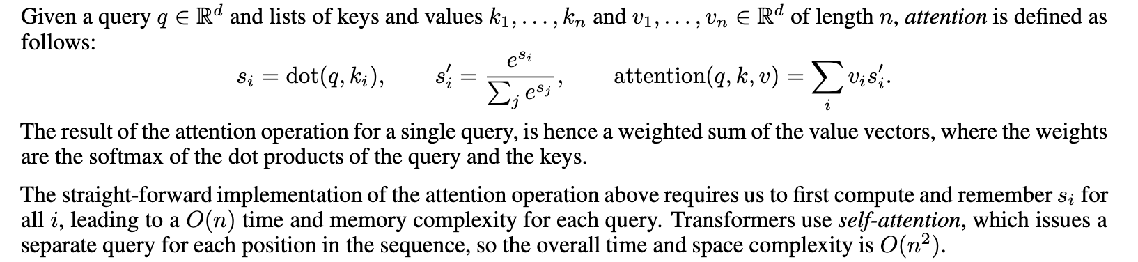
Paying attention to Attention heads

Why another attention post

There are a lot of tutorials out there explaining attention mechanism with illustrations.

Two of my favorites are

• Understanding and coding Self attention mechanism of large language models from Scratch

• The illustrated transformer

After reading the paper Attention is all you need and the articles mentioned above, I was curious about:

1. Projecting the embedded space into a feature subspace and subsequent learning of these spaces during training.

2. Scaled self-attention, why scale the value.

3. Finally the Big O of computing pairwise score. Space and time complexity.

I will pass on the burden of deciding about the triviality of these observations to the readers.

Background

It is easy to understand attention as a feature selection exercise. Not all input features seen by a model are equally important for the task at hand. Prudence dictates we make the model pay more attention to important features than considering all the features presented to it.

1. For each feature, compute importance score. The higher the score, the more critical the feature.
2. Use these scores in downstream tasks to guide the model.

Some example concepts implementing the above steps:

• Lasso regression, l1 regularization ensures that some of the model coefficients are pushed towards zero.

• Maxpooling layers in CNN selects’ the cell with maximum values and ignore the rest of cell values.

In both instances above, a feature is either retained or discarded according to its importance score. It’s worth noting that these importance scores have the potential to enhance the information conveyed by the feature. The goal of attention is to enrich the information the feature carries. Attention mechanism digs into the context of the given feature and make them context-aware.

Context awareness

“Try to infer the meaning of the word based on its neighbors” - Many amongst us have heard this during our elementary reading classes.

In sequential features, in addition to individual elements, the relationship among the elements carries a lot of information. This relationship is called the context.

• In the sentence “premature optimization is the root cause of all evil,” the famous Donald Knuth quote, the word evil is better understood from the context of “premature optimization.”

• In a time series sales data, the sales of this quarter is related to the previous quarter.

• In image data, the neighboring pixels are correlated.

• In video data, pixel from the current frames can be enriched with the information from previous frames.

Attention is a way of enriching the features, making the features context-aware.

Attention bare bones

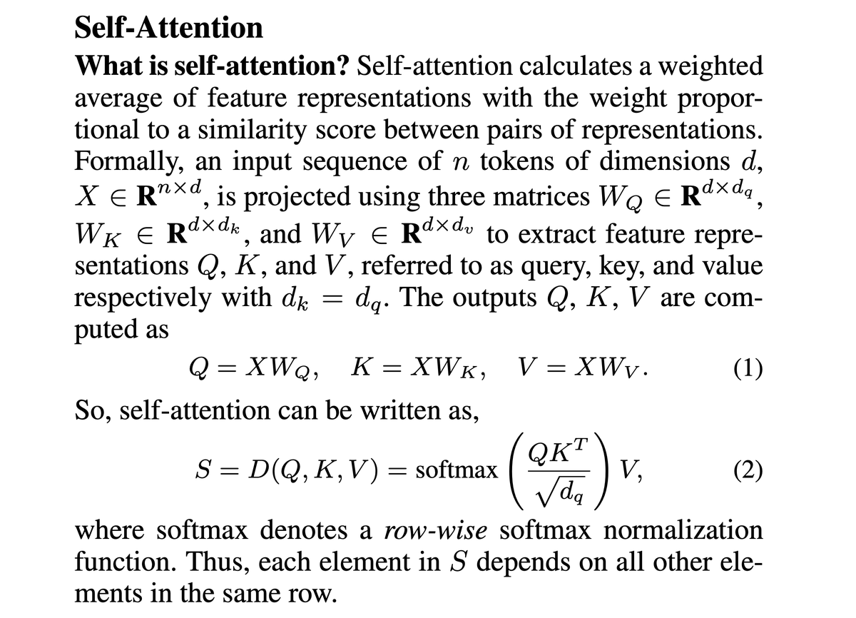
We will focus on the scaled dot product attention proposed in the paper Attention is all you need.

Its easy to comprehend (for me!) the context-aware phenomenon when the inputs are a list of words; basic input units to any natural language processing task.

In the sentence “John plays ukulele occasionally”, we expect that for the token “John”, the most related word token should be “plays”. We expect to enrich the feature representation for token “John” with its relation to the token “plays”.

A standard text preprocessing looks like the below figure.

Without going into the details of each of these blocks, let us pretend we took the output of embedding block.

import numpy as np

SEQ_LEN   = 5
EMBD_LEN  = 10

x = np.random.normal(size=(SEQ_LEN,EMBD_LEN))

The input is a matrix of size (5 x 10), where each row represents the embedding of a word token, a total of 5 word tokens.

Why embeddings

In 2003 Yoshua Bengio and his team introduced embeddings in the paper, A neural probabilistic language model. Journal of Machine Learning Research, 3:1137-1155, 2003. Since then several follow up research and development occurred in the embedding space.

For our purpose to continue with the rest of the article, word embeddings are a representation of words in a vector space. They map the language into a structured geometric space. Geometric relation between two word vectors will hence reflect the semantic relationship between them. We can leverage linear algebra techniques to find similarity between words.

I personally like the 2013 google paper Efficient estimation of word representations in vector space. This paper introduces CBOW and Skip-ngram architecture to learn word representations from large corpus. An example from this paper, arithmetic operations performed on word vectors,

Paris - France + Italy = Rome.

Subracting the vector for France from Paris and adding the vector for Italy, gives a vector which is very close to Rome.

Pair-wise scoring aka attenion scores

Here we find the similarity between words using dot product.

For the initiated, to keep things simple, I have ignored scaling and softmax normalization. Will take it up in the following sections.

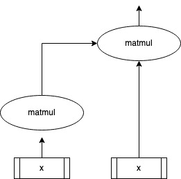
pairwise_scoring = np.matmul(x,x.T)

Each word is a vector.We use the dot product similarity to find the pair-wise scoring between the words. An illustration of pair wise calculation¹.

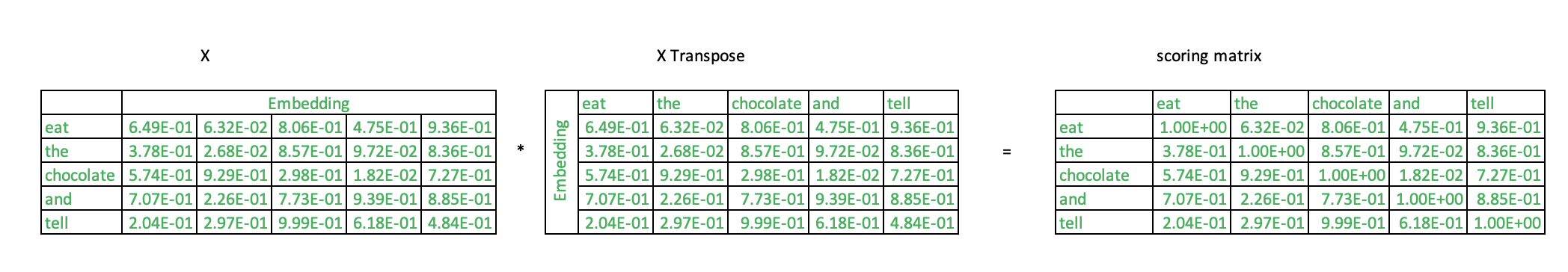
These pairwise scores are called attention scores. Word close to each another in the geometric space, will have a higher attention score.

The resultant pairwise_scoring is a 5 x 5 matrix which encodes the attention scores between these words.

Enrich the input with attention score

In the above diagram, the row gives attention scores for word eat with the other words in the input. Enriching is performing of a weighted sum of the individual word embedding vectors with the attention scores.

The attention score for the word ‘eat’ and ‘eat’ is multiplied with ‘eat’ vector. The score for word ‘the’ and ‘eat’ is multiplied with ‘the’ vector and son on. Finally we add all these vectors to get the final enriched vector for the word ‘eat’. Words which are semantically close to “eat” will contribute more and others will contribute less.

enriched_x_ = np.zeros(shape=x.shape)
for i, scores in enumerate(pairwise_scoring):
    weighted_sum = np.zeros(x[0,:].shape)
    for j,score in enumerate(scores):
        weighted_sum+= x[j,:] * score
    enriched_x[i] = weighted_sum

We can vectorize the above operation.

enriched_x = np.matmul(pairwise_scoring,x)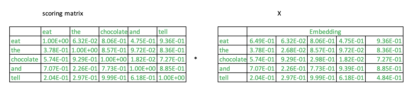

Voila

This is the underlying idea behind attention. Since the words are represented in the vector space, dot product of the vectors provides the similarity scores between words. Semantically similar words will have high attention scores and finally will contribute more to word in question through weighted sum.

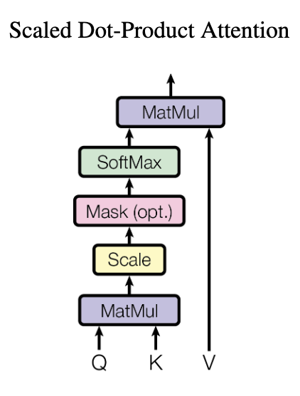
Scaled dot product attention

Here is a great tweet from hardmaru succinctly explaining self attention.

In the rest of the section, we will pretty much dwell into the contents of this tweet.

With a fair understanding of the attention score calculation, let us compare what we have learned in the previous section with the scaled dot product attention mechanism proposed in attention is all you need paper.

In the table above, the first column has the picture from Attention is all you need paper. The second column depicts our bare bone attention explained in the previous section.

1. Bare bone had a single input X, our word embeddings matrix. The scaled dot attention has three inputs, Q,K,V.

2. What are the additional boxes, scale, mask and softmax in scaled dot-product attention.

Query, Key, Value Model

Let us address the first question. All blogs and papers refer to input as Q,K and V. This comes from the search engine / recommendation terminology. Going back in history to early days of search engine, inverted indices was the data structure which powered searches on large databases.

Documents were indexed based on words. An entry in an inverted index can be imagined as Key,Value pair as shown,

{keyword1,keyword21,keyword45}:{Document1,Document100,Document121}

This kind of indexing accelerates keyword based searches.

Let us say the whole vocabulary is a set, V = {keyword1,….keywordm}; m keywords; and the document corpus is D ={Document1,…Documentn} ; n documents

Given a query, Q = {keyword1,keyword20,keyword21}. We can retrieve all the all documents containing the key word query as follows

results = sum( intersection(Q, K) * V) for all n Documents

vocabulary = ['a','b','c','d']
documents  = ['d1','d2', 'd3','d4','d5']

inverted_index = {('a','b'): ['d1','d2']
                 ,('a','c'): ['d1','d2','d3']
                 ,('b'): ['d1','d2']
                 ,('c','d'): ['d4','d5']
                 }

query = ('a','c')


results = set()
for key,value in inverted_index.items():
    match = set(query).intersection(set(key))
    if  len(match) >= 1:
        for document in value:
            results.add(document)

The function intersection(Q, K) can be replaced by a scoring function instead of a discrete intersection. Imaging our pairwise_scoring replacing this function.

While explaining the bare bones attention, our input played the role of Query, Key, and Value. There is no rule that Query, Key, and Value should be three different inputs. When same input is used for query, key and value, its called as self-attention.

Attention is a feature enhancement mechanism to improve the downstream applications. Query, Key,Value model is a comfortable way to explain the input of different downstream tasks like search, sequence to sequence learning, language models, and others. Hence Query, Key, and Value representation are used while describing attention.

Why do the transformation

In most of papers, Q, K and V are transformations of the input matrix. Original input matrix is not directly used to calculate attention scores. In the following code, wqp, wkp and wvp are equivalent to Q, K and V matrices depicted in the diagram.

q_d = k_d = 20 # dimension of query and key weights
v_d = 25       # dimension of value matrix weight

wq = np.random.normal(size=(q_d, EMBD_LEN))
wk = np.random.normal(size=(k_d, EMBD_LEN))
wv = np.random.normal(size=(v_d, EMBD_LEN))

wqp = np.matmul(wq,x.T).T
wkp = np.matmul(wk,x.T).T
wvp = np.matmul(wv,x.T).T

Three random weight matrices, wq,wk and wv are created. These matrices are used to project input matrix x to create three new matrices, wqp, wkp and wvp. The input shapes of all the participating matrices are given below,

x, input shape (5, 10)
wq, q weight matrix shape (20, 10)
wk, k weight matrix shape (20, 10)
wv, v weight matrix shape (25, 10)

wqp, q weight matrix shape (5, 20)
wkp, k weight matrix shape (5, 20)
wvp, v weight matrix shape (5, 25)

The initial input matrix x, with dimension 5 x 10 is now projected into three new matrices. In wqp and wkp the embedded space of dimension 10 is projected into a feature space of dimension 20. In wvp its projected into a space of dimension 25.

Why not use the input matrix x directly as we did in the bare bone attention example ?

• While doing the pair-wise scoring on the input matrix, you notice that the diagonal values of the resultant matrix is all 1. This would mean that we are instructing the model to attend to the current word more. After projection this may not be the case.

• The matrices wq,wk and wv serve as a parameter to the final neural network and will be adjusted based on gradients during back propagation. This will allow the network to learn the new feature space. I always had this question about the importance of word embeddings for downstream natural language processing tasks. Had recently put a survey in linked in. Clicke here for the survey Say we are building a classifier on a corpus of engineering notes written by a technician servicing an aircraft. The lingo and word tokens are going to reflect the domain. Previously trained embeddings may not have a corresponding word vectors.

In such scenarios do we resort to create an embedding space for that vocabulary before we build our classifier? There are no clear pragmatic rules. However, by projecting some of these embeddings into another subspace, we hope that transformers or other dense network ingesting these projected matrices will learn those geometric mapping during the training process.

In worst case, the bytepair encoding or sentencepair encoding may split some of these words in a way we don’t want. The downstream learning may become completely useless, as a words split badly may be mapped to wrong geometric spaces.

Masking

Neural networks mandates fixed length inputs. While working on natural language tasks, we achieve this by fixing the input length to a constant value. If the number of word tokens in the input is greater than this fixed value, we trim it. If the word tokens fall short of the fixed value, we pad them with null values.

While calculating the attention score, we don’t want to include the padded entries in the calculation. Hence the mask.

Calculate the self-attention

Finally we calculate the self-attention. In a nutshell we find the similarity between the items in our matrices. We have projected 5 words from embedded space to a new feature space, we find the similarity between these five word tokens.

score = np.matmul(wqp, wkp.T)
scaled_score = score / np.sqrt(wkd)

The resultant matrix, score is a 5 x 5 matrix.

The dot product can get very large, hence the scaling. From the paper Attention is all you need, the foot note explains the need for scaling.

“To illustrate why the dot products get large, assume that the components of q and k are independent random variables with mean 0 and variance 1. Their dot product will have a mean of 0 and variance of dk”

More importantly we need to keep the magnitude of the dot product controlled because of the subsequent application of softmax.

def softmax(x):
    e_x = np.exp(x)
    return e_x / e_x.sum(axis=1,keepdims=True)

scaled_softmax_score = softmax(scaled_score)

Without scaling, applying softmax on very large value can lead to arithmetic computation problem. Exponent of large numbers can result in very large values. Softmax normalizes the attention scores.

Finally the attention context vector is created as follows. The weighted sum of the input and corresponding attention scores.

context_vector = np.sum(np.matmul(scaled_softmax_score, wvp),axis=0)

We have the context vector which is context aware, thanks to self attention mechanism.

Space and time complexity.

Space time complexity of pure attention calculation is O(n^2), where n is number of word tokens.

Look at the extract from paper Self-Attention does not need O(n^2) memory

The above paper proposes a constant memory and logarithmic memory. The division of exponential summation is moved following the distributive law as shown in the figure below from the paper.

The quadratic time complexity is a good motivation for further research. Reformer: The effiecient transfomer replaces dot product attention with locality-sensitive hashing, changing the complexity from quadratic to log.

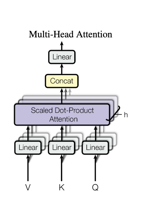
Multi-head Attention

From attention is all you need paper, “Instead of performing a single attention function with keys, values and queries, we found it beneficial to linearly project the queries, keys and values h times with different, learned linear projections. On each of these projected versions of queries, keys and values we then perform the attention function in parallel, yielding output values. These are concatenated and once again projected.”

The query, key and values are projected through three different learned matrices. Attention scores derived from the query and key projection matrices, is applied to the values projection matrix. A single context vector is the output. This forms a single head. Multiple such heads are constructed and the context vectors from these heads are concatenated together and projected one final time.

Finally

Started the article with three questions,

1. Projecting the embedded space into a feature subspace and subsequent learning of these spaces during training.

2. Scaled self-attention, why scale the value.

3. Finally the Big O of computing pairwise score. Space and time complexity.

We discussed about the need for projection and how the Query,Key and Value model serve as the projected space. Projection allows the model to learn the nuances of the input space for the task in hand. Since the embedding space was trained on a completely different corpus, it may not encode the similarities in an expected manner.

By scaling, we control the magnitude of the attention scores and avoid subsequent arithmetic problems which can creep when softmax is applied.

Finally to cover the Space and time complexity of attention, we glanced over the recent works by Google to tackle the space complexity and a new architecture called as Reformer to tackle the time complexity.

1. The resultant scoring matrix was filled with random numbers. Apologies to those meticulous readers who actually multiplied these matrices. ↩